TESS Planet Finding App

Core of the project: a model to CATEGORIZE light-curves

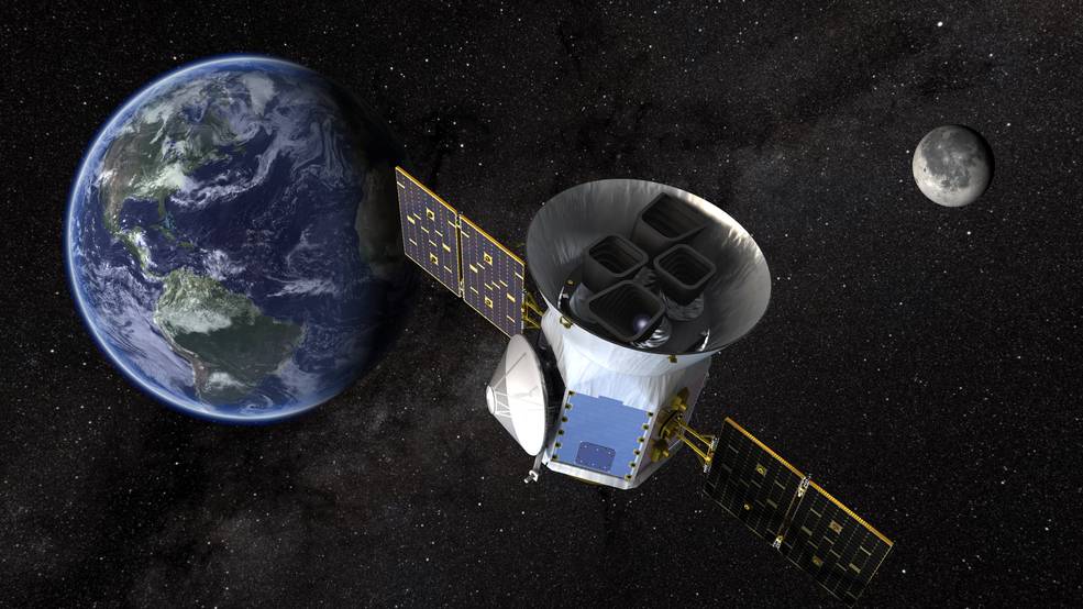
NASA's TESS satellite started taking light readings of 200,000 of the brightest, closest stars in 2018. Nasa expects to find about 300 earth-sized exoplanets within the next year. Data from this on-going project is being made available to the public. For my very first co-op project, another Data Science student and I paired up to see if we could find anything interesting.

To be clear, neither of us are astrophysicists. Nonetheless, after brainstorming together, we came up with a way for a way that machine learning might contribute to NASA's project without any reference to physics. To train a classification model, all we needed was a set of data to train on both with and without exoplanets - think hotdog / not a hotdog from the show Silicon Valley. We had access to the raw data without any classification. If we could get a list of stars in the data that had already been established as likely to have planets, then we were in business.

As it turned out, CalTech had already begun composing a list of most likely stars in the TESS data to have planets. They wanted to get this information out there to direct the attention of the physics community towards the stars that were most likely to yield interesting results, and to get people to start pointing equipment in the right directions. As it so happened, this is exactly the information we also needed to build a classification model.

We combined the CalTech data with data from STScI in Baltimore, MD, together the data formed X and y vectors of our models. We also found a number of helpful Jupyter Notebooks on the community resources section of NASA's website to create nice light-curve visuals like the one below.

Essentially, our model took in the whole swath of these scattered data-points for each planet and was charged to produce a single probability for whether each star had at least one planet. The power of this approach, though it could never stand alone, is that it allows us to look for patterns that we were not looking for explicitly. While initially physics might find probable planets in the data using rigid and well defined rules, our secondary / piggy-back approach allowed us to look for general patterns. Most notably, we are not really able to say exactly what the patterns are that our model is picking up on, only that it must be catching on to something if it is predicting accurately.

Part 1: GETTING DATA AND VISUALIZING IT

Getting data from CalTech:

import pandas as pd

# Getting labelled TESS Objects of Interest df from Caltech:
toi = pd.read_csv('https://exofop.ipac.caltech.edu/tess/' + 
					'download_toi.php?sort=toi&output=csv')

# Isolating columns of interest:
toi = toi[['TIC ID',
			'TOI',
			'Epoch (BJD)',
			'Period (days)',
			'Duration (hours)',
			'Depth (mmag)',
			'Planet Radius (R_Earth)',
			'Planet Insolation (Earth Flux)',
			'Planet Equil Temp (K)',
			'Planet SNR',
			'Stellar Distance (pc)',
			'Stellar log(g) (cm/s^2)',
			'Stellar Radius (R_Sun)',
			'TFOPWG Disposition',
			]]
#some cleaning
toi.columns = toi.columns.str.replace(' ', '_')

Getting data from STScI:

from astroquery.mast import Catalogs
from astropy.table import Table
from tqdm import tqdm

# Getting additional data on TESS Objects of Interest from STScI:
tic_catalog = pd.DataFrame()
for tic_id in tqdm(toi['TIC_ID'].unique()):
	row_data = Catalogs.query_criteria(catalog="Tic", ID=tic_id)
	row_data = row_data.to_pandas()
	tic_catalog = tic_catalog.append(row_data)
tic_catalog = tic_catalog.reset_index(drop=True)

# Renaming ID column to make this consistent with Caltech TOI dataframe:
tic_catalog = tic_catalog.rename(columns={'ID': 'TIC_ID'})

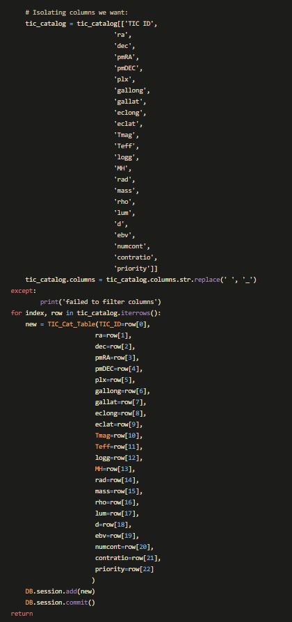
# Isolating columns of interest:
tic_catalog = tic_catalog[['TIC_ID',
			'ra',
			'dec',
			'pmRA',
			'pmDEC',
			'plx',
			'gallong',
			'gallat',
			'eclong',
			'eclat',
			'Tmag',
			'Teff',
			'logg',
			'MH',
			'rad',
			'mass',
			'rho',
			'lum',
			'd',
			'ebv',
			'numcont',
			'contratio',
			'priority']]

tic_catalog.columns = tic_catalog.columns.str.replace(' ', '_')

Getting dataproduct URLs for stars in the dataframes above cataloged by TIC id from STScI:

from astroquery.mast import Observations

# Getting all dataproducts for TESS Objects of Interest from STScI:
dataproducts = pd.DataFrame()
for tic_id in tqdm(toi['TIC_ID'].unique()):
	row_data = Observations.query_criteria(obs_collection="TESS",
											target_name=tic_id)
	row_data = row_data.to_pandas()
	dataproducts = dataproducts.append(row_data)
dataproducts = dataproducts.reset_index(drop=True)

# Renaming ID column to make this consistent with Caltech TOI dataframe:
dataproducts = dataproducts.rename(columns={'target_name': 'TIC_ID'})

# Isolating TIC IDs (target_name) and dataURL values to get associated files:
dataproducts = dataproducts[['TIC_ID', 'dataURL']]

dataproducts.columns = dataproducts.columns.str.replace(' ', '_')

To inspect the uniqueness of dataproducts available for each star (TIC id):

# Getting list of unique TIC IDs in each of the three dataframes:
toi_unique_ids = toi['TIC_ID'].unique().tolist()
tic_catalog_unique_ids = tic_catalog['TIC_ID'].unique().tolist()
dataproducts_unique_ids = dataproducts['TIC_ID'].unique().tolist()
dataproducts_unique_ids = [int(tic_id) for tic_id in dataproducts_unique_ids]

After exploring the above resulting lists, it was time to try to extract some information. Relying heavily on tutorials found through the NASA community pages (See here)  , the following yield all light-curves from an example star:

from astropy.io import fits
import matplotlib.pyplot as plt

# Getting urls for all dataproducts associated with TIC ID 29781292:
urls_for_29781292 = dataproducts[dataproducts['TIC_ID'] == '29781292'][
	'dataURL'].tolist()

# Getting urls for all lc.fits files associated with TIC ID 29781292:
lcs_for_29781292 = [url for url in urls_for_29781292 if 
					url.endswith('lc.fits')]

# Describing and plotting all lc.fits files associated with TIC ID 29781292:
# See https://github.com/spacetelescope/notebooks/blob/master/notebooks/
# MAST/TESS/beginner_how_to_use_lc/beginner_how_to_use_lc.ipynb
for url in lcs_for_29781292:
	
	fits_file = ('https://mast.stsci.edu/api/v0.1/Download/file?uri=' + url)
	
	# print(fits.info(fits_file), "\n")
	
	# print(fits.getdata(fits_file, ext=1).columns)
	
	with fits.open(fits_file, mode="readonly") as hdulist:
		tess_bjds = hdulist[1].data['TIME']
		sap_fluxes = hdulist[1].data['SAP_FLUX']
		pdcsap_fluxes = hdulist[1].data['PDCSAP_FLUX']
	
	fig, ax = plt.subplots()

	ax.plot(tess_bjds, pdcsap_fluxes, 'ko')

	ax.set_ylabel("PDCSAP Flux (e-/s)")
	ax.set_xlabel("Time (TBJD)")

	plt.show()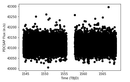

For the sample star chosen for this example there were another 12 plots like the one above plotted from the code block above. Some stars had several dataproducts, while others had none.

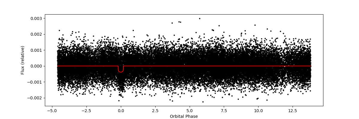
For most stars, the data plots below were also available. Again, information for how to do this was found here

import numpy as np

# Getting urls for all dvt.fits files associated with TIC ID 29781292:
# dvts_for_29781292 = [url for url in urls_for_29781292 if 
# url.endswith('dvt.fits')]

# Describing and plotting all lc.fits files associated with TIC ID 29781292:
# See https://github.com/spacetelescope/notebooks/blob/master/notebooks/MAST/
# TESS/beginner_how_to_use_dvt/beginner_how_to_use_dvt.ipynb
for url in dvts_for_29781292:

fits_file = ('https://mast.stsci.edu/api/v0.1/Download/file?uri=' + url)

print(fits.info(fits_file), "\n")

print(fits.getdata(fits_file, ext=1).columns)

with fits.open(fits_file, mode="readonly") as hdulist:

	star_teff = hdulist[0].header['TEFF']
	star_logg = hdulist[0].header['LOGG']
	star_tmag = hdulist[0].header['TESSMAG']

	period = hdulist[1].header['TPERIOD']
	duration = hdulist[1].header['TDUR']
	epoch = hdulist[1].header['TEPOCH']
	depth = hdulist[1].header['TDEPTH']

	times = hdulist[1].data['TIME']
	phases = hdulist[1].data['PHASE']
	fluxes_init = hdulist[1].data['LC_INIT']
	model_fluxes_init = hdulist[1].data['MODEL_INIT']

sort_indexes = np.argsort(phases)

fig, ax = plt.subplots(figsize=(12,4))

ax.plot(phases[sort_indexes], fluxes_init[sort_indexes], 'ko',
		markersize=2)

ax.plot(phases[sort_indexes], model_fluxes_init[sort_indexes], '-r')

ax.set_ylabel("Flux (relative)")
ax.set_xlabel("Orbital Phase")

plt.show()

This produces all of the dvt light-curve plots available for a star in the TESS data. An example dvt plot:

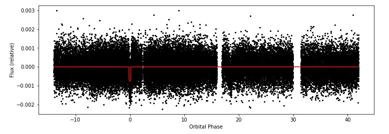
Finally, we could save our newly wrangled data in new csv files:

toi.to_csv('toi_example.csv')
tic_catalog.to_csv('tic_catalog_example.csv')
dataproducts.to_csv('dataproducts_example.csv')

PART 2: BUILDING A PREDICTIVE MODEL

Since we were going to need to get our data into a SQL database, we started by pulling our csv data saved above into a pandas df, transferred it into a sqlite db, then back into a pandas df, merged on the unique star number (TIC id).

from sqlalchemy import create_engine
from astropy.io import fits

# Importing example data:
toi = pd.read_csv('toi_example.csv')
tic_catalog = pd.read_csv('tic_catalog_example.csv')

# Getting it into an sqlite database:
engine = create_engine('sqlite://', echo=False)

toi.to_sql('toi', con=engine, index=False)
tic_catalog.to_sql('tic_catalog', con=engine, index=False)
# Pulling data from sql database:
toi = pd.read_sql_table('toi', engine).drop(columns='Unnamed: 0')
tic_catalog = pd.read_sql_table(
	'tic_catalog', engine).drop(columns='Unnamed: 0')

# Assembling data needed for model:
df = toi.merge(tic_catalog, on='TIC_ID')

Next came some data cleaning and a Test/Train split. In this case, because the size of the training set was relatively small, we decided against a validation split.

from sklearn.model_selection import train_test_split

# Separating confirmed planets from false positives:
df['TFOPWG_Disposition'] = df[
	'TFOPWG_Disposition'].replace({'KP': 1, 'CP': 1, 'FP': 0})

# Creating confirmed planets dataframe:
cp_df = df[df['TFOPWG_Disposition'] == 1]

# Creating false positives dataframe:
fp_df = df[df['TFOPWG_Disposition'] == 0]

# Train/test split on both dataframes:
cp_train, cp_test = train_test_split(cp_df, random_state=42)
fp_train, fp_test = train_test_split(fp_df, random_state=42)

# Combining training dataframes:
train = cp_train.append(fp_train)
train = train.sample(frac=1, random_state=42).reset_index(drop=True)

# Combining test dataframes:
test = cp_test.append(fp_test)
test = test.sample(frac=1, random_state=42).reset_index(drop=True)

# Dropping columns from training dataframe that aren't used in model:
X_train = train.drop(columns=['TIC_ID', 'TOI', 'TFOPWG_Disposition'])
# Getting labels for training data:
y_train = train['TFOPWG_Disposition'].astype(int)

# Dropping columns from test dataframe that aren't used in model:
X_test = test.drop(columns=['TIC_ID', 'TOI', 'TFOPWG_Disposition'])
# Getting labels for test data:
y_test = test['TFOPWG_Disposition'].astype(int)

Finally it was time to build a Keras Neural Network model:

from tensorflow import keras
from tensorflow.keras.models import Sequential
from tensorflow.keras.layers import Dense
from tensorflow.keras import optimizers
from tensorflow.keras.wrappers.scikit_learn import KerasClassifier
from sklearn.preprocessing import RobustScaler
from sklearn.impute import SimpleImputer
from sklearn.pipeline import make_pipeline

# Setting up model architecture for neural net:
def create_model():
	# Instantiate model:
	model = Sequential()
	# Add input layer:
	model.add(Dense(20, input_dim=33, activation='relu'))
	# Add hidden layer:
	model.add(Dense(20, activation='relu'))
	# Add output layer:
	model.add(Dense(1, activation='sigmoid'))
	# Compile model:
	model.compile(loss='binary_crossentropy', optimizer='adam',
				metrics=['accuracy'])
	return model

# Putting neural net in a pipeline:
pipeline = make_pipeline(
	SimpleImputer(strategy='mean'),
	RobustScaler(),
	KerasClassifier(build_fn=create_model, verbose=2)
)

# Fitting the neural net:
pipeline.fit(X_train,
				y_train,
				kerasclassifier__batch_size=5,
				kerasclassifier__epochs=50,
				kerasclassifier__validation_split=.2,
				kerasclassifier__verbose=2)

# Printing train and test accuracy:
print('\n\n')
print(f'Train Accuracy Score:', pipeline.score(X_train, y_train), '\n')
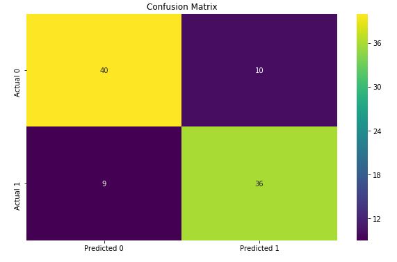
print(f'Test Accuracy Score:', pipeline.score(X_test, y_test))

After running 50 epochs, accuracy honed in on about 80% with a loss around 1.08:

Part 3: Building our Model into an App

In addition to building the model itself, my DS partner and I set out to create a simple interactive app with our findings. As a minimal product, we hoped for a user to be able to select a star from the data and see a light-curve graph with our model's predictions.

To tackle this, I built a Python Flask App. In retrospect, we really didn't need to reproduce all of our work in the app, but we did. I created a number of python classes in Object Oriented Programming style to most easily transfer our local work on a sqlite database to a populating our production PostgreSQL DB and used SQLAlchemy. The idea was to build something that we could come back to and build out more features.

from flask_sqlalchemy import SQLAlchemy

#Instantiate
DB = SQLAlchemy()

# create visualization info class
class Visual_Table(DB.Model):
	id = DB.Column(DB.Integer, primary_key=True)
	TIC_ID = DB.Column(DB.BigInteger, nullable=False)
	dataURL = DB.Column(DB.String(100))
	def __repr__(self):
	return ''.format(self.TIC_ID)

class TOI_Table(DB.Model):
	id = DB.Column(DB.Integer, primary_key=True)
	TIC_ID = DB.Column(DB.BigInteger, nullable=False)
	TOI = DB.Column(DB.Float)
	Epoch = DB.Column(DB.Float)
	Period = DB.Column(DB.Float)
	Duration = DB.Column(DB.Float)
	Depth = DB.Column(DB.Float)
	Planet_Radius = DB.Column(DB.Float)
	Planet_Insolation = DB.Column(DB.Float)
	Planet_Equil_Temp = DB.Column(DB.Float)
	Planet_SNR = DB.Column(DB.Float)
	Stellar_Distance = DB.Column(DB.Float)
	Stellar_log_g = DB.Column(DB.Float)
	Stellar_Radius = DB.Column(DB.Float)
	TFOPWG_Disposition = DB.Column(DB.String)
	def __repr__(self):
	return ''.format(self.TIC_ID)

class TIC_Cat_Table(DB.Model):
	id = DB.Column(DB.Integer, primary_key=True)
	TIC_ID = DB.Column(DB.BigInteger, nullable=False)
	ra = DB.Column(DB.Float)
	dec = DB.Column(DB.Float)
	pmRA = DB.Column(DB.Float)
	pmDEC = DB.Column(DB.Float)
	plx = DB.Column(DB.Float)
	gallong = DB.Column(DB.Float)
	gallat = DB.Column(DB.Float)
	eclong = DB.Column(DB.Float)
	eclat = DB.Column(DB.Float)
	Tmag = DB.Column(DB.Float)
	Teff = DB.Column(DB.Float)
	logg = DB.Column(DB.Float)
	MH = DB.Column(DB.Float)
	rad = DB.Column(DB.Float)
	mass = DB.Column(DB.Float)
	rho = DB.Column(DB.Float)
	lum = DB.Column(DB.Float)
	d = DB.Column(DB.Float)
	ebv = DB.Column(DB.Float)
	numcont = DB.Column(DB.Float)
	contratio = DB.Column(DB.Float)
	priority = DB.Column(DB.Float)
	def __repr__(self):
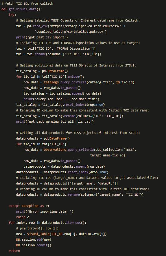
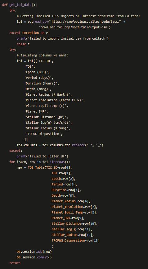
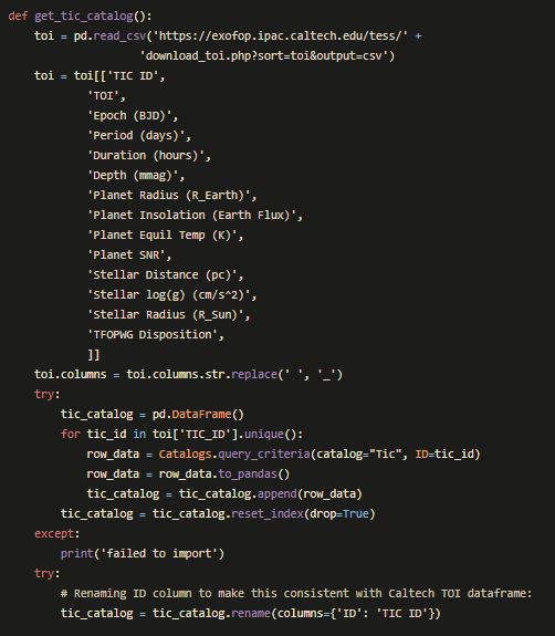
	return ''.format(self.TIC_ID)

To populate this database, I created three functions to live in a .py file to fetch data for our three tables above. The nearly 200 lines of code of these functions can be found: https://github.com/mikedcurry/TESS_Flask_App/blob/master/App_TESS/Data_in.py

The long code-block below does essentially the same thing as in the Jupyter Notebook exerpt from Part 1 above. The difference here is that it uses OOP techniques to populate a SQL database. Everything is built into functions so that we can later build the routes to call them in the main .py file or our app.

With the architecture of our database set out, and our model built into a callable function, we were ready to spend the last day of the project creating all the routes in our Flask App.

def create_app():
"""create and config an instance of the Flask App"""
app = Flask(__name__)

# configure DB, will need to update this when changing DBs?
app.config['SQLALCHEMY_DATABASE_URI'] = config('DATABASE_URL')
app.config['SQLALCHEMY_TRACK_MODIFICATIONS'] = False
app.config['ENV'] = config('ENV')
DB.init_app(app)
# with app.app_context():
#     db.create_all()

# Create home route
@app.route('/')
def root():
	#Pull example data from Notebooks folder. Will be be pulled from sql DB in the future.
	return render_template('home.html', 
				title = 'Finding Planets:TESS', 
				toi_table=(TOI_Table.query.all()), 
				tic_table=(TIC_Cat_Table.query.all())
				)     

@app.route('/total_reset')
def total_reset():
	DB.drop_all()
	DB.create_all()
	get_visual_data()
	get_toi_data()
	get_tic_catalog()
	return render_template('home.html', title='Reset Database!')

@app.route('/predict')
def predict():
	get_all_predictions()
	return render_template('home.html', title='prediction pipeline works!')

return app

It doesn't look like much yet, but we got a web app deployed. Our PostgreSQL database is populated, and we have a functioning pipeline for our model. On the front end, which was built over the course of about two hours with virtually no experience with HTML at the time, there is a table with a set of links to go to the light curve graphs.

Check out the deployed app. Be patient, it takes a few seconds to load. :D

• Deployed App